Quickstart
I want to use CCA or PLS. How many samples are required?
Simply import gemmr
In [1]: from gemmr import *
Then, for CCA, only the number of features in each of the 2 datasets needs to be specified, e.g.
In [2]: cca_sample_size(100, 50)
Out[2]: {0.1: 83427, 0.3: 6562, 0.5: 2012}
The result is a dictionary with keys indicating assumed ground truth correlations and values giving the corresponding sample size estimate. For PLS, in addition to the number of features in each dataset the powerlaw decay constant for the within-set principal component spectrum needs to be specified:
In [3]: pls_sample_size(100, 50, -1.5, -.5)
Out[3]: {0.1: 236437, 0.3: 32769, 0.5: 13074}
Note
Required sample sizes are calculated to obtain at least 90% power and less than 10% error in a number of other metrics. See the [gemmr] publication for more details.
More use cases and options of the sample size functions are discussed in Sample size calculation.
How can I generate synthetic data for CCA or PLS?
The functionality is provided in module generative_model and requires two steps
In [4]: from gemmr.generative_model import setup_model, generate_data
First, a model needs to be specified. The required parameters are:
- the number of features in X and Y
- the assumed true correlation between scores in X and Y
- the power-law exponents describing the within-set principal component spectra of X and Y
In [5]: px, py = 3, 5

In [6]: r_between = 0.3

In [7]: ax, ay = -1, -.5

In [8]: Sigma = setup_model('cca', px=px, py=py, ax=ax, ay=ay, r_between=r_between)
Analogously, if a model for PLS is desired the first argument becomes 'pls'.
Second, given the model, data can be drawn from the normal distribution associated with the covariance matrix Sigma:
In [9]: X, Y = generate_data(Sigma, px, n=5000)

In [10]: X.shape, Y.shape
Out[10]: ((5000, 3), (5000, 5))
See the API reference for generative_model.setup_model() and generative_model.generate_data() for more details.
How do the provided CCA or PLS estimators work?
We assume two data arrays X and Y are given and shall be analyzed with CCA or PLS. The provided estimators
work like those in sklearn. For example, to perform a CCA:
In [11]: from gemmr.estimators import SVDCCA

In [12]: cca = SVDCCA(n_components=1)

In [13]: cca.fit(X, Y)
Out[13]: SVDCCA()
After fitting several attributes become available. Estimated canonical correlations are stored in
In [14]: cca.corrs_
Out[14]: array([0.30308498, 0.04694188, 0.01331049])
weight (rotation) vectors in
In [15]: cca.x_rotations_
Out[15]:
array([[0.18886894],
       [0.68264445],
       [0.70592144]])
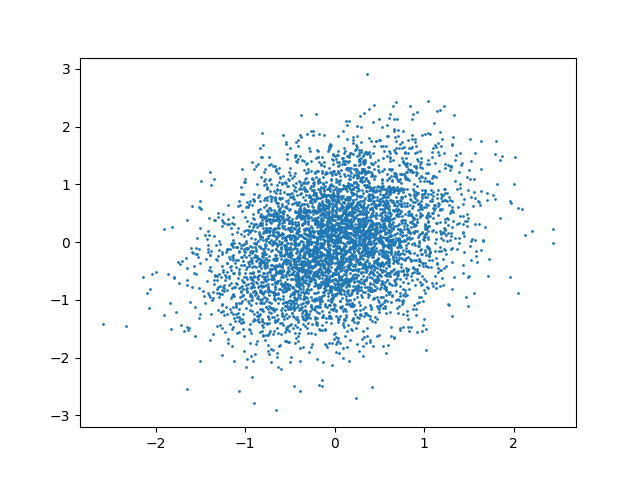
and analogously in cca.y_rotations_, and the attributes x_scores_ and y_scores_ provide the in-sample scores:
In [16]: plt.scatter(cca.x_scores_, cca.y_scores_, s=1)
Out[16]: <matplotlib.collections.PathCollection at 0x7f82d8e3b4e0>
SVDPLS works analogously, but note that it finds maximal covariances instead of correlations, and correspondingly has an attribute covs_.
For more information see the reference pages for estimators.SVDCCA and estimators.SVDPLS.
A sparse CCA estimator, based on the R-package PMA, is implemented as estimators.SparseCCA.
How can I investigate parameter dependencies of CCA or PLS?
This can be done with the function sample_analysis.analyze_model_parameters().
A basic use case is shown here:
In [17]: from gemmr.sample_analysis import *

In [18]: results = analyze_model_parameters(
   ....:     'cca',
   ....:     pxs=(2, 5), rs=(.3, .5), n_per_ftrs=(2, 10, 30, 100),
   ....:     n_rep=10, n_perm=1,
   ....: )
   ....:

In [19]: results
Out[19]:
<xarray.Dataset>
Dimensions:                     (Sigma_id: 1, mode: 1, n_per_ftr: 4, perm: 1, px: 2, r: 2, rep: 10, x_feature: 5, x_orig_feature: 5, y_feature: 5, y_orig_feature: 5)
Coordinates:
  * y_orig_feature              (y_orig_feature) int64 0 1 2 3 4
  * r                           (r) float64 0.3 0.5
  * Sigma_id                    (Sigma_id) int64 0
  * n_per_ftr                   (n_per_ftr) int64 2 10 30 100
  * x_orig_feature              (x_orig_feature) int64 0 1 2 3 4
  * x_feature                   (x_feature) int64 0 1 2 3 4
  * y_feature                   (y_feature) int64 0 1 2 3 4
  * px                          (px) int64 2 5
Dimensions without coordinates: mode, perm, rep
Data variables:
    between_assocs              (px, r, Sigma_id, n_per_ftr, rep) float64 0.5856 ... 0.4817
    between_covs_sample         (px, r, Sigma_id, n_per_ftr, rep) float64 0.2379 ... 0.3608
    between_corrs_sample        (px, r, Sigma_id, n_per_ftr, rep) float64 0.5856 ... 0.4817
    x_weights                   (px, r, Sigma_id, n_per_ftr, rep, x_feature, mode) float64 -0.7755 ... 0.5364
    y_weights                   (px, r, Sigma_id, n_per_ftr, rep, y_feature, mode) float64 -0.9897 ... -0.6565
    x_loadings                  (px, r, Sigma_id, n_per_ftr, rep, x_orig_feature, mode) float64 -0.7337 ... 0.4976
    y_loadings                  (px, r, Sigma_id, n_per_ftr, rep, y_orig_feature, mode) float64 -0.9197 ... -0.6245
    between_assocs_perm         (px, r, Sigma_id, n_per_ftr, rep, perm) float64 0.8095 ... 0.1353
    between_covs_sample_perm    (px, r, Sigma_id, n_per_ftr, rep, perm) float64 0.3596 ... 0.1024
    between_corrs_sample_perm   (px, r, Sigma_id, n_per_ftr, rep, perm) float64 0.8095 ... 0.1353
    x_weights_perm              (px, r, Sigma_id, n_per_ftr, rep, perm, x_feature, mode) float64 -0.9788 ... -0.3067
    y_weights_perm              (px, r, Sigma_id, n_per_ftr, rep, perm, y_feature, mode) float64 -0.9975 ... -0.4528
    x_loadings_perm             (px, r, Sigma_id, n_per_ftr, rep, perm, x_orig_feature, mode) float64 -0.9671 ... -0.2974
    y_loadings_perm             (px, r, Sigma_id, n_per_ftr, rep, perm, y_orig_feature, mode) float64 -0.9882 ... -0.4158
    between_assocs_true         (px, r, Sigma_id, mode) float64 0.3 0.5 0.3 0.5
    x_weights_true              (px, r, Sigma_id, x_feature, mode) float64 -0.4642 ... 0.5642
    y_weights_true              (px, r, Sigma_id, y_feature, mode) float64 -0.9942 ... -0.672
    ax                          (px, r, Sigma_id) float64 -0.6454 ... -0.2939
    ay                          (px, r, Sigma_id) float64 -0.257 ... -0.1957
    latent_expl_var_ratios_x    (px, r, Sigma_id, mode) float64 0.4374 ... 0.1808
    latent_expl_var_ratios_y    (px, r, Sigma_id, mode) float64 0.5434 ... 0.1924
    weight_selection_algorithm  (px, r, Sigma_id) <U4 'qr__' 'qr__' ... 'qr__'
    x_loadings_true             (px, r, Sigma_id, x_feature, mode) float64 -0.5482 ... 0.5354
    x_crossloadings_true        (px, r, Sigma_id, x_feature, mode) float64 -0.1645 ... 0.2677
    y_loadings_true             (px, r, Sigma_id, y_feature, mode) float64 -0.9951 ... -0.6408
    y_crossloadings_true        (px, r, Sigma_id, y_feature, mode) float64 -0.2985 ... -0.3204
    py                          (px) int64 2 5
The variable results contains a number of outcome metrics by default,
and further ones can be obtained through add-ons specified
as keyword-argument addons to sample_analysis.analyze_model_parameters().
Dependence of outcomes on, for example, sample size, can then be inspected:
In [20]: plt.loglog(results.n_per_ftr, results.between_assocs.sel(px=5, r=0.3, Sigma_id=0).mean('rep'), label='r=0.3')
Out[20]: [<matplotlib.lines.Line2D at 0x7f82d8e3bda0>]

In [21]: plt.loglog(results.n_per_ftr, results.between_assocs.sel(px=5, r=0.5, Sigma_id=0).mean('rep'), label='r=0.5')
Out[21]: [<matplotlib.lines.Line2D at 0x7f82d8e2f898>]

In [22]: plt.xlabel('samples per feature')
Out[22]: Text(0.5, 0, 'samples per feature')

In [23]: plt.ylabel('canonical correlation')
Out[23]: Text(0, 0.5, 'canonical correlation')

In [24]: plt.legend()
Out[24]: <matplotlib.legend.Legend at 0x7f82d8f22f98>

In [25]: plt.gcf().tight_layout()
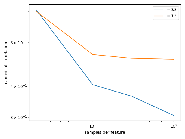
See Model parameter analysis for a more extensive example and the reference page for
sample_analysis.analyzers.analyze_model_parameters() for more details.