Overview
What are CCA and PLS?
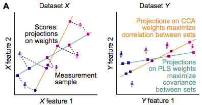
Canonical Correlation Analysis (CCA) and Partial Least Squares (PLS) are methods that reveal associations between multivariate datasets. Commonly, associations are assessed with (e.g.) the Pearson correlation coefficient between two features. When datasets have a multitude of features, however, pairwise associations focus on only narrow aspects in the data and multivariate methods that take into account all features at the same time can be advantageous. CCA and PLS do that by determining weighted composites of the features such that the association strength between the weighted composites is optimal: CCA maximizes the correlation, PLS maximizes the covariance.
What problems can occur with CCA and PLS?
When only a small number of samples are available, CCA and PLS can overfit the data. To demonstrate this, we use an example dataset
In [1]: from sklearn.datasets import load_linnerud

In [2]: X, Y = load_linnerud(return_X_y=True)

In [3]: X.shape, Y.shape
Out[3]: ((20, 3), (20, 3))
CCA determines weights for each feature such that the weighted sums of features in both datasets correlate maximally.
Solely to be able to illustrate better the resulting weights, let us use use only 2 of the three features in X
In [4]: X = X[:, :2]
and perform CCA on random subsamples of small size
In [5]: from gemmr.estimators import SVDCCA

In [6]: cca = SVDCCA()

In [7]: n_iter = 3000

In [8]: n_subsamples = 6

In [9]: np.random.seed(0)

In [10]: x_weights_6 = np.empty((n_iter, 2))

In [11]: corrs_6 = np.empty(n_iter)

In [12]: for i in range(n_iter):
   ....:     inds = np.random.permutation(len(X))[:n_subsamples]
   ....:     cca.fit(X[inds], Y[inds])
   ....:     corrs_6[i] = cca.corrs_[0]
   ....:     x_weights_6[i] = cca.x_rotations_[:, 0]
   ....:
And, for comparison, we’re repeating the same analysis using 12 instead of 6 samples in each iteration
In [13]: n_subsamples = 12

In [14]: x_weights_12 = np.empty((n_iter, 2))

In [15]: corrs_12 = np.empty(n_iter)

In [16]: for i in range(n_iter):
   ....:     inds = np.random.permutation(len(X))[:n_subsamples]
   ....:     cca.fit(X[inds], Y[inds])
   ....:     corrs_12[i] = cca.corrs_[0]
   ....:     x_weights_12[i] = cca.x_rotations_[:, 0]
   ....:
Let’s now look at the estimated canonical correlations
In [17]: plt.violinplot([corrs_6, corrs_12])
Out[17]:
{'bodies': [<matplotlib.collections.PolyCollection at 0x7f224062f400>,
  <matplotlib.collections.PolyCollection at 0x7f224062f760>],
 'cmaxes': <matplotlib.collections.LineCollection at 0x7f224062f2e0>,
 'cmins': <matplotlib.collections.LineCollection at 0x7f224062fd30>,
 'cbars': <matplotlib.collections.LineCollection at 0x7f2240642100>}

In [18]: plt.ylabel('estimated canonical correlation')
Out[18]: Text(0, 0.5, 'estimated canonical correlation')

In [19]: plt.xticks([1, 2], ['6 samples', '12 samples'])
Out[19]:
([<matplotlib.axis.XTick at 0x7f224058bca0>,
  <matplotlib.axis.XTick at 0x7f224058bc70>],
 [Text(1, 0, '6 samples'), Text(2, 0, '12 samples')])
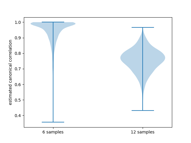
When CCA was performed on samples of size 6 the estimated canonical correlations almost always were essentially 1! This seems unrealistic in practice and in fact when the sample size is doubled estimated canonical correlations drop noticably. Beyond that, it’s not clear what canonical correlations we would get if we had a larger (or infinite) sample size at our disposal. This aspect of how canonical correlations depend on sample size is further investigated in the Analyses from paper.
Let’s now look at the estimated weight vectors. Note that CCA weights are ambiguous with respect to their signs. Therefore, for consistency, we here arbibtrarily choose the signs of the weights such that the second element of the weight vectors is positive
In [20]: x_weights = x_weights_12

In [21]: x_weights *= np.sign(x_weights[:, [1]])
Then, we can illustrate the weights
In [22]: import matplotlib.pyplot as plt

In [23]: plt.scatter(x_weights[:, 0], x_weights[:, 1], s=5)
Out[23]: <matplotlib.collections.PathCollection at 0x7f2240223eb0>

In [24]: plt.gca().set_aspect(1)
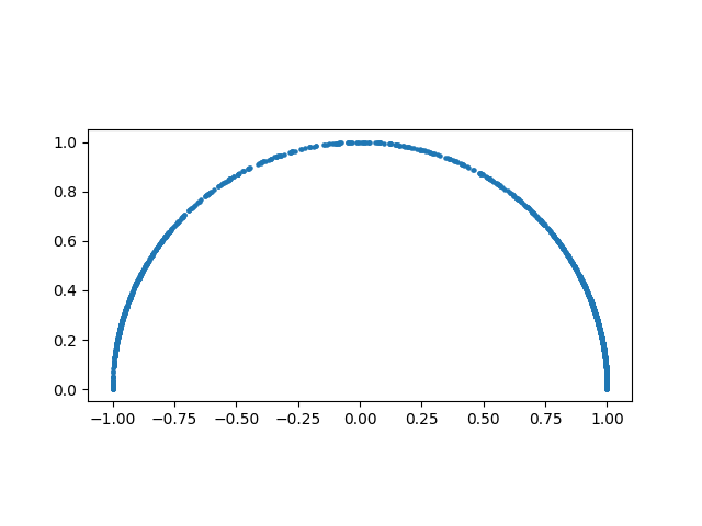
Each point in this plot represents a weight vector. As each of the 2-dimensional weight vectors are normalized to unit length they necessarily need to lie on a circle with radius 1. What’s surprising here, is that the weight vectors cover the whole circle (semi-circle, as the second element was constrained to be positive). This means that the estimated weight vector can be every possible weight vector, depending on which particular data sample was measured. I.e., the inferred weights are completely unreliable in this scenario. As for the canonical correlations, it is unclear what weight vectors we would obtain if we had a larger (or infinite) data sample. However, for CCA to be useful, i.e. for the weights to be interpretable, we need reliable weight estimates.
To obtain reliable estimates for the canonical correlations and weight vectors, samples of sufficient size are required and gemmr provides functionality to determine this size.
What does gemmr do?
gemmr assists in determining an appropriate sample size for a CCA or PLS analysis. It does so by generating synthetic data, performing CCA / PLS on the synthetic data sample and evaluating how close the results are to the truth. To that end, gemmr provides functionality to
generate synthetic data with known parameter dependencies
perform CCA and PLS
evaluate parameter dependencies of CCA / PLS results
determine appropriate sample sizes
The main parameters of interest on which CCA / PLS results depend and which are needed to generate synthetic data are
the dimensionality of the data
the assumed true association strength between weighted composites of the datasets
the within-set variance structure, i.e. the principal component variance spectrum in each dataset
the sample size
For more information, see How it works, Analyses from paper, as well as the [gemmr] publication.
Helmer et al., On stability of Canonical Correlation Analysis and Partial Least Squares with application to brain-behavior associations, bioRxiv, 2020. DOI: 10.1101/2020.08.25.265546. https://www.biorxiv.org/content/10.1101/2020.08.25.265546v1