Quickstart
I want to use CCA or PLS. How many samples are required?
Simply import gemmr
In [1]: from gemmr import *
Then, for CCA, only the number of features in each of the 2 datasets, as well as the powerlaw decay constant for the within-set principal component spectrum, need to be specified, e.g.
In [2]: cca_sample_size(100, 50, -.8, -1.2)
Out[2]: {0.1: 189701, 0.3: 17211, 0.5: 5638}
The result is a dictionary with keys indicating assumed ground truth correlations and values giving the corresponding sample size estimate. For PLS, sample size can be calculated similarly:
In [3]: pls_sample_size(100, 50, -1.5, -.5)
Out[3]: {0.1: 331230, 0.3: 52919, 0.5: 22555}
Note
Required sample sizes are calculated to obtain at least 90% power and less than 10% error in a number of other metrics. See the [gemmr] publication for more details.
More use cases and options of the sample size functions are discussed in Sample size calculation.
How can I generate synthetic data for CCA or PLS?
The functionality is provided in module generative_model and requires two steps
In [4]: from gemmr.generative_model import GEMMR
First, a model needs to be specified. The required parameters are:
the number of features in X and Y
the assumed true correlation between scores in X and Y
the power-law exponents describing the within-set principal component spectra of X and Y
In [5]: px, py = 3, 5

In [6]: r_between = 0.3

In [7]: ax, ay = -1, -.5

In [8]: gm = GEMMR('cca', wx=px, wy=py, ax=ax, ay=ay, r_between=r_between)
Analogously, if a model for PLS is desired the first argument becomes 'pls'.
Second, data can be drawn from the model distribution:
In [9]: X, Y = gm.generate_data(n=5000)

In [10]: X.shape, Y.shape
Out[10]: ((5000, 3), (5000, 5))
See the API reference for generative_model.setup_model() and generative_model.generate_data() for more details.
How do the provided CCA or PLS estimators work?
We assume two data arrays X and Y are given and shall be analyzed with CCA or PLS. The provided estimators
work like those in sklearn. For example, to perform a CCA:
In [11]: from gemmr.estimators import SVDCCA

In [12]: cca = SVDCCA(n_components=1)

In [13]: cca.fit(X, Y)
Out[13]: SVDCCA()
After fitting several attributes become available. Estimated canonical correlations are stored in
In [14]: cca.corrs_
Out[14]: array([0.27596667])
weight (rotation) vectors in
In [15]: cca.x_rotations_
Out[15]:
array([[-0.87806565],
       [-0.11246735],
       [-0.46513633]])
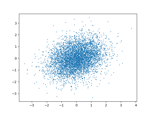
and analogously in cca.y_rotations_, and the attributes x_scores_ and y_scores_ provide the in-sample scores:
In [16]: plt.scatter(cca.x_scores_, cca.y_scores_, s=1)
Out[16]: <matplotlib.collections.PathCollection at 0x7f224142edc0>
SVDPLS works analogously, but note that it finds maximal covariances instead of correlations, and correspondingly has an attribute covs_.
For more information see the reference pages for estimators.SVDCCA and estimators.SVDPLS.
A sparse CCA estimator, based on the R-package PMA, is implemented as estimators.SparseCCA.
How can I investigate parameter dependencies of CCA or PLS?
This can be done with the function sample_analysis.analyze_model_parameters().
A basic use case is shown here:
In [17]: from gemmr.sample_analysis import *

In [18]: results = analyze_model_parameters(
   ....:     'cca',
   ....:     pxs=(2, 5), rs=(.3, .5), n_per_ftrs=(2, 10, 30, 100),
   ....:     n_rep=10, n_perm=1,
   ....: )
   ....:

In [19]: results
Out[19]:
<xarray.Dataset>
Dimensions:                    (x_feature: 5, y_feature: 5, n_per_ftr: 4,
                                Sigma_id: 1, r: 2, px: 2, rep: 10, mode: 1,
                                perm: 1)
Coordinates:
  * x_feature                  (x_feature) int64 0 1 2 3 4
  * y_feature                  (y_feature) int64 0 1 2 3 4
  * n_per_ftr                  (n_per_ftr) int64 2 10 30 100
  * Sigma_id                   (Sigma_id) int64 0
  * r                          (r) float64 0.3 0.5
  * px                         (px) int64 2 5
Dimensions without coordinates: rep, mode, perm
Data variables: (12/25)
    between_assocs             (px, r, Sigma_id, n_per_ftr, rep) float64 0.88...
    between_covs_sample        (px, r, Sigma_id, n_per_ftr, rep) float64 0.52...
    between_corrs_sample       (px, r, Sigma_id, n_per_ftr, rep) float64 0.88...
    x_weights                  (px, r, Sigma_id, n_per_ftr, rep, x_feature, mode) float64 ...
    y_weights                  (px, r, Sigma_id, n_per_ftr, rep, y_feature, mode) float64 ...
    x_loadings                 (px, r, Sigma_id, n_per_ftr, rep, x_feature, mode) float64 ...
    ...                         ...
    ay                         (px, r, Sigma_id) float64 -1.0 -1.0 -1.0 -1.0
    x_loadings_true            (px, r, Sigma_id, x_feature, mode) float64 0.9...
    x_crossloadings_true       (px, r, Sigma_id, x_feature, mode) float64 0.2...
    y_loadings_true            (px, r, Sigma_id, y_feature, mode) float64 0.5...
    y_crossloadings_true       (px, r, Sigma_id, y_feature, mode) float64 0.1...
    py                         (px) int64 2 5
Attributes:
    model:           cca
    estr:            SVDCCA(calc_loadings=True, cov_out_of_bounds='raise')
    powerlaw_decay:  (-1, -1)
    created:         2023-12-04 01:54:36.753119
    gemmr_version:   0+unknown
The variable results contains a number of outcome metrics by default,
and further ones can be obtained through add-ons specified
as keyword-argument addons to sample_analysis.analyze_model_parameters().
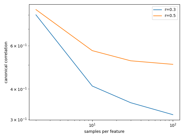
Dependence of outcomes on, for example, sample size, can then be inspected:
In [20]: plt.loglog(results.n_per_ftr, results.between_assocs.sel(px=5, r=0.3, Sigma_id=0).mean('rep'), label='r=0.3')
Out[20]: [<matplotlib.lines.Line2D at 0x7f2241439850>]

In [21]: plt.loglog(results.n_per_ftr, results.between_assocs.sel(px=5, r=0.5, Sigma_id=0).mean('rep'), label='r=0.5')
Out[21]: [<matplotlib.lines.Line2D at 0x7f224070f850>]

In [22]: plt.xlabel('samples per feature')
Out[22]: Text(0.5, 0, 'samples per feature')

In [23]: plt.ylabel('canonical correlation')
Out[23]: Text(0, 0.5, 'canonical correlation')

In [24]: plt.legend()
Out[24]: <matplotlib.legend.Legend at 0x7f224070f610>

In [25]: plt.gcf().tight_layout()
See Model parameter analysis for a more extensive example and the reference page for
sample_analysis.analyzers.analyze_model_parameters() for more details.