Analysis of prior literature

Here, we look into CCAs reported in the literature. We analyze sample-size dependence of reported association strengths and estimate the corresopnding weight errors.

Setup

import numpy as np
import pandas as pd
import xarray as xr

from sklearn.linear_model import LinearRegression

from gemmr.metrics import mk_weightError
from gemmr.data import load_outcomes, print_ds_stats, load_metaanalysis, load_metaanalysis_outcomes

import holoviews as hv
from holoviews import opts, dim
hv.extension('matplotlib')
hv.renderer('matplotlib').param.set_param(dpi=120)

from my_config import *

import warnings
# holoviews emits this for log-linear plots
warnings.filterwarnings(
    'ignore', 'aspect is not supported for Axes with xscale=log, yscale=linear', category=UserWarning
)
warnings.filterwarnings(
    'ignore', 'aspect is not supported for Axes with xscale=linear, yscale=log', category=UserWarning
)

# This will be populated below and then written to disk
plotted_data = {}

CCAs in literature

metaanalysis_data = load_metaanalysis()

metaanalysis_data.columns

Index(['PMID', 'Title', 'Authors', 'Citation', 'First Author', 'Journal/Book',
       'Publication Year', 'Create Date', 'PMCID', 'NIHMS ID', 'DOI',
       'CCA variant', 'n', 'n unit', 'subject_groups', 'is_healthy', 'dataset',
       'n_sites', 'brain-behavior association', 'X modality', 'Y modality',
       'pX', 'pY', 'Comment', 'latent association stengths reported', 'r1'],
      dtype='object')

We’re extracting studies that used CCA to analyze brain-behavior relationships, and reported the used sample size, the number of features in the data and the estimated canonical correlation

def try_float(r):
    try:
        return float(r)
    except:
        return np.nan


cond_cca_bba = (
    (metaanalysis_data['CCA variant'] == 'CCA') &
    (metaanalysis_data['brain-behavior association'] == 'yes')
)
cond_npr = (
    np.isfinite(metaanalysis_data['n'].apply(try_float)) &
    np.isfinite(metaanalysis_data['pX'].apply(try_float)) &
    np.isfinite(metaanalysis_data['pY'].apply(try_float)) &
    np.isfinite(metaanalysis_data['r1'].apply(try_float))
)


metaanalysis_data_ = metaanalysis_data[cond_cca_bba & cond_npr].copy()
metaanalysis_data_.loc[:, 'r1'] = metaanalysis_data_['r1'].astype(float)
metaanalysis_data_.loc[:, 'pX'] = metaanalysis_data_['pX'].astype(int)
metaanalysis_data_.loc[:, 'pY'] = metaanalysis_data_['pY'].astype(int)
metaanalysis_data_.loc[:, 'n'] = metaanalysis_data_['n'].astype(int)

assert len(metaanalysis_data_['DOI']) == len(metaanalysis_data_['DOI'].dropna())

How popular has CCA been in the brain-behavior literature over time? For this analysis only we consider all CCA studies, independent of if they reported sample size, number of features and canonical correlation.

pub_years = metaanalysis_data[cond_cca_bba]['Publication Year'].groupby(metaanalysis_data[cond_cca_bba]['DOI']).mean().values
hist, edges = np.histogram(pub_years, bins=np.arange(pub_years.min(), pub_years.max()+2))
panel_nCCAStudies_by_year = hv.Histogram(
    (edges, hist)
).redim(
    x='Year',
    Frequency='Num CCA studies of\nbrain behavior associations'
).opts(*fig_opts).opts(
    opts.Histogram(fig_inches=(1.7, None))
)

hv.save(panel_nCCAStudies_by_year, 'fig/figS_nCCAStudies_by_year.pdf')

panel_nCCAStudies_by_year

From here on, we only consider studies that do report sample size, number of features and canonical correlation. How many are there?

print('n_publications =', len(metaanalysis_data_['DOI'].unique()))
print('n_CCAs =', len(metaanalysis_data_))

n_publications = 31
n_CCAs = 100

Let’s see how many samples per feature studies typically use (if a publication reports several CCAs with the same number of samples and the same number of features for both datasets we count it as one here)

n_per_ftrs = []
for doi, df in metaanalysis_data_.groupby('DOI'):
    n_per_ftrs += (df['n'] / (df['pX'] + df['pY'])).unique().tolist()
n_per_ftrs = np.array(n_per_ftrs)

# # Alternatively, count each reported CCA, even if it there are multiple ones from the same study
# # with the same number of samples and the same number of features in both datasets
# n_per_ftrs = (metaanalysis_data_['n'] / (metaanalysis_data_['pX'] + metaanalysis_data_['pY']))

log_n_per_ftrs = np.log(n_per_ftrs)

bins = np.sort(list(set(np.logspace(0, log_n_per_ftrs.max()*1.01, 10, base=np.exp(1), dtype=int).tolist())))
bins = np.log(bins)
counts, bins = np.histogram(log_n_per_ftrs, bins=bins, density=False)
bins = np.exp(bins)

panel_n_per_ftr_hist = hv.Histogram(
    ((bins, counts))
).redim(
    x='Samples per feature',
    Frequency='Num. reported CCAs'
).opts(*fig_opts).opts(
    opts.Histogram(logx=True, fig_inches=(1.7, None), xlim=(1, 100)),
)

# hv.save(panel_n_per_ftr_hist, 'fig/figS_metaanalysis_n_per_ftr_histogram.pdf')

panel_n_per_ftr_hist

Let’s also see how the reported canonical correlations relate to the samples-per-feature of the used data:

def is_healthy_marker(s):
    if s == 'yes':
        return 's'
    # elif s == 'no':
    #     return 'x'
    else:
        return 'd'
marker = metaanalysis_data_['is_healthy'].apply(is_healthy_marker)

metaanalysis_n_per_ftr = (metaanalysis_data_['n'].astype(float) / (metaanalysis_data_['pX'].astype(float) + metaanalysis_data_['pY'].astype(float)))

panel_metaanalysis_rObs_nPerFtr = hv.Overlay()
for my_marker in np.unique(marker):
    mask = (marker == my_marker)
    panel_metaanalysis_rObs_nPerFtr *= hv.Scatter(
        (metaanalysis_n_per_ftr[mask], metaanalysis_data_['r1'][mask]),
        kdims=['Samples per feature'],
        vdims='Canonical corr.',
        # label='Literature',
    ).opts(*fig_opts).opts(
        logx=True, logy=True, color='black', s=10, fig_inches=(1.7, None), marker=my_marker
    )

# save plotted data
_plotted_data = pd.DataFrame(
    metaanalysis_data_['r1'][mask].values,
    index=metaanalysis_n_per_ftr[mask].values
)
_plotted_data.columns = ['r']
_plotted_data.index.names = ['n_per_ftr']
plotted_data['CCAs_in_literature'] = _plotted_data

panel_metaanalysis_rObs_nPerFtr.opts(*fig_opts).opts(
    fig_inches=(1.7, None)
)

This looks pretty linear. What’s the corresponding \(R^2\) value?

X = np.log(metaanalysis_n_per_ftr.values.reshape(-1, 1))
y = np.log(metaanalysis_data_['r1'].values)

lm = LinearRegression(fit_intercept=True).fit(X, y)
log_nPerFtr_obsCorr_R2 = lm.score(X, y)
log_nPerFtr_obsCorr_R2

0.833416333963024

What’s the relation between canonical correlation and samples per feature in synthetic data with known true correlation?

data_home = None
ds_cca = load_outcomes('sweep_cca_cca_0+0_litanaDenseSweep', data_home=data_home)

Loading data from subfolder 'gemmr_latest'

What’s in the simulated outcome data file?

print_ds_stats(ds_cca)

n_modes          1
n_rep            100
n_perm           10
n_per_ftr        [  3   4   6   8  12  16  24  32  48  64  96 100]
r                [0.1 0.3 0.5]
px               [  2   4   8  16  32  64 128]
ax+ay range     (0.00, 0.00)
py              == px

<xarray.DataArray 'n_Sigmas' (px: 7, r: 3)>
array([[10, 10, 10],
       [10, 10, 10],
       [10, 10, 10],
       [10, 10, 10],
       [10, 10, 10],
       [10, 10, 10],
       [10, 10, 10]])
Coordinates:
  * r        (r) float64 0.1 0.3 0.5
  * px       (px) int64 2 4 8 16 32 64 128

power           not calculated

What’s the relation between observed canonical correlation and samples per feature in synthetic data?

panel_synthetic = hv.Overlay()
_r_clrs = ['grey'] + hv.Palette(cmap_r, samples=3).values

_plotted_data = {}

_ds_perm = ds_cca.between_assocs_perm \
    .mean('perm').mean('rep').mean('px').mean('Sigma_id').mean('r')
_plotted_data['perm'] = _ds_perm.to_dataframe()['between_assocs_perm']
panel_synthetic *= hv.Curve(
    (_ds_perm.n_per_ftr, _ds_perm.values), label='perm'
).opts(
    logx=True, logy=True
)

for r in ds_cca.r.values:
    _ds = ds_cca.between_assocs.sel(r=r).mean('rep').mean('px').mean('Sigma_id')
    _plotted_data[r] = _ds.drop('r').to_dataframe()['between_assocs']
    panel_synthetic *= hv.Curve(
        (_ds.n_per_ftr, _ds.values),
        label='$r=%.1f$' % r
    ).opts(
        logx=True, logy=True
    )

# save plotted data
_plotted_data = pd.concat(_plotted_data, axis=1)
_plotted_data.columns.names = ['r_true']
plotted_data['simulated_observed_correlations'] = _plotted_data


panel_synthetic *= hv.Text(1, 0.1, '0.5', halign='left', valign='bottom', fontsize=8).opts(color=_r_clrs[-1])
panel_synthetic *= hv.Text(1, 0.1*1.3, '0.3', halign='left', valign='bottom', fontsize=8).opts(color=_r_clrs[-2])
panel_synthetic *= hv.Text(1, 0.1*1.3*1.3, '0.1', halign='left', valign='bottom', fontsize=8).opts(color=_r_clrs[-3])
panel_synthetic *= hv.Text(1, 0.1*1.3*1.3*1.3, 'perm', halign='left', valign='bottom', fontsize=8).opts(color=_r_clrs[-4])
panel_synthetic *= hv.Text(1, 0.1*1.3*1.3*1.3*1.3, '$r_\mathrm{true}=$', halign='left', valign='bottom', fontsize=8)

panel_synthetic = panel_synthetic.redim(
    x='Samples per feature',
    y='Observed correlation'
).opts(*fig_opts).opts(
    opts.Curve(color=hv.Cycle(_r_clrs)),
    opts.Overlay(logx=True, logy=True, show_legend=False, fig_inches=(1.7, None), yticks=3),
)
panel_synthetic

Now, let’s compare literature to synthetic data

fig = panel_synthetic * panel_metaanalysis_rObs_nPerFtr
fig.opts(*fig_opts).opts(fig_inches=(1.7, None), show_legend=False)

Estimate weight errors for reported CCAs

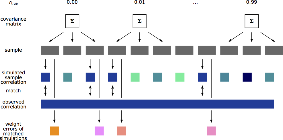
To estimate the weight errors for a reported CCA we use the number of features of the reported CCA, repeatedly generate synthetic data of the same sample size as the reported CCA, and sweep through the assumed true correlations. For each synthetic dataset we perform CCA. Whenever the estimated canonical correlation in the synthetic data matches the reported canonical correlation we calculate and record the weight error in the synthetic dataset. We then use the collection of recorded synthetic weight errors as an estimate for the weight error in the reported CCA.

Following the description above, we have generate synthetic data for each combination of \(p_X, p_Y\) and \(n\) in our database and analyzed it with gemmr. The resulting datasets look, for example, like this:

print_ds_stats(load_metaanalysis_outcomes(px=8, py=7, n=95, data_home=data_home))

n_modes          1
n_rep            100
n_per_ftr        [6]
r                [0.   0.01 0.02 0.03 0.04 0.05 0.06 0.07 0.08 0.09 0.1  0.11 0.12 0.13
 0.14 0.15 0.16 0.17 0.18 0.19 0.2  0.21 0.22 0.23 0.24 0.25 0.26 0.27
 0.28 0.29 0.3  0.31 0.32 0.33 0.34 0.35 0.36 0.37 0.38 0.39 0.4  0.41
 0.42 0.43 0.44 0.45 0.46 0.47 0.48 0.49 0.5  0.51 0.52 0.53 0.54 0.55
 0.56 0.57 0.58 0.59 0.6  0.61 0.62 0.63 0.64 0.65 0.66 0.67 0.68 0.69
 0.7  0.71 0.72 0.73 0.74 0.75 0.76 0.77 0.78 0.79 0.8  0.81 0.82 0.83
 0.84 0.85 0.86 0.87 0.88 0.89 0.9  0.91 0.92 0.93 0.94 0.95 0.96 0.97
 0.98 0.99]
px               [8]
ax+ay range     (0.00, 0.00)
py              != px

<xarray.DataArray 'n_Sigmas' (px: 1, r: 100)>
array([[1, 1, 1, 1, 1, 1, 1, 1, 1, 1, 1, 1, 1, 1, 1, 1, 1, 1, 1, 1, 1, 1,
        1, 1, 1, 1, 1, 1, 1, 1, 1, 1, 1, 1, 1, 1, 1, 1, 1, 1, 1, 1, 1, 1,
        1, 1, 1, 1, 1, 1, 1, 1, 1, 1, 1, 1, 1, 1, 1, 1, 1, 1, 1, 1, 1, 1,
        1, 1, 1, 1, 1, 1, 1, 1, 1, 1, 1, 1, 1, 1, 1, 1, 1, 1, 1, 1, 1, 1,
        1, 1, 1, 1, 1, 1, 1, 1, 1, 1, 1, 1]])
Coordinates:
  * r        (r) float64 0.0 0.01 0.02 0.03 0.04 ... 0.95 0.96 0.97 0.98 0.99
  * px       (px) int64 8

power           not calculated

The following piece of code performs the second part of the analysis: it finds synthetic datasets with estimated canonical correlation matching the empirical one and calculates the corresponding weight error in the synthetic dataset:

def get_error(n, px, py, target_corr, calc_error_fun=mk_weightError, error_kind=.975,
              corr_bw=0.1, qs=(.025, .5, .975), verbose=False):

    if (px == 1) or (py == 1):
        return np.nan

    ds = load_metaanalysis_outcomes(px, py, n)

    corr_cond = np.abs(ds.between_assocs / target_corr - 1) < corr_bw
    if corr_cond.sum() == 0:
        return np.nan

    if verbose:
        print(n, px, py, target_corr, 'n_corr_cond =', int(corr_cond.sum()))

    error = calc_error_fun(ds)
    conditional_error = error.where(corr_cond)

    if error_kind == 'distribution':
        return conditional_error

    else:
        error_stats = xr.concat([
            conditional_error.quantile(qs),
            xr.DataArray([conditional_error.mean()], dims=('quantile',), coords=dict(quantile=['mean'])),
        ],
            'quantile'
        )
        res = error_stats.sel(quantile=error_kind)
        if res.ndim == 0:
            res = float(res)
        return res

weight_errors = [
    get_error(row[1]['n'], row[1]['pX'], row[1]['pY'], row[1]['r1'],
              calc_error_fun=mk_weightError, error_kind='mean')
    for row in metaanalysis_data_.iterrows()
]
metaanalysis_data_['mean_estimated_weight_error'] = weight_errors

Let’s overlay the estimated weight errors on the observed-correlation vs samples-per-feature plot:

def is_healthy_marker(s):
    if s == 'yes':
        return 's'
    elif s == 'no':
        return 'd'
    else:
        return 'x'
marker = metaanalysis_data_['is_healthy'].apply(is_healthy_marker)

panel_metaanalysis_rObs_nPerFtr = hv.Overlay()
for my_marker in np.unique(marker):
    mask = (marker == my_marker)
    panel_metaanalysis_rObs_nPerFtr *= hv.Scatter(
        (metaanalysis_n_per_ftr[mask], metaanalysis_data_['r1'][mask],
        metaanalysis_data_['mean_estimated_weight_error'][mask].rename('Estim_weight_error')),
        kdims=['Samples per feature'],
        vdims=['Observed correlation', 'Estim weight error'],
    ).opts(*fig_opts).opts(
        fig_inches=(1.7, None), s=20, edgecolor='black', linewidth=.25, logx=True, logy=True,
        color=dim('Estim_weight_error'), cmap='PuRd', colorbar=True, clim=(.0, 1), clabel='Estim. weight error', marker=my_marker
    )

panel_metaanalysis_rObs_nPerFtr.opts(*fig_opts).opts(
    fig_inches=(5, None)
)

panel_metaanalysis_rObs_nPerFtr = hv.Scatter(
    (metaanalysis_n_per_ftr, metaanalysis_data_['r1'],
     metaanalysis_data_['mean_estimated_weight_error'].rename('Estim_weight_error')),
    kdims=['Samples per feature'],
    vdims=['Observed correlation', 'Estim weight error'],
    label='Analysis of prior literature',
).opts(*fig_opts).opts(
    fig_inches=(1.7, None), s=10, marker='o', edgecolor='black', linewidth=.25, logx=True, logy=True,
    color=dim('Estim_weight_error'), cmap='PuRd', colorbar=True, clim=(.0, 1), clabel='Estim. weight error'
)

panel_metaanalysis_rObs_nPerFtr

We’re going to look at two more aspects of the estimated weight errors:

• What’s the distribution of estimated weight errors for a given reported CCA?

• It appears that the weight errors are smaller the farther a point (i.e. a reported CCA) lies away from the top-left to bottom-right diagonal in the plot. We’ll look more closely at this relationship

Distribution of weight errors

weight_error_distribs = [
    get_error(row[1]['n'], row[1]['pX'], row[1]['pY'], row[1]['r1'],
              calc_error_fun=mk_weightError, error_kind=slice(None), qs=(.025, .975), verbose=True)
    for row in metaanalysis_data_.iterrows()
]

assert isinstance(weight_error_distribs[0], xr.DataArray)
for i in range(len(weight_error_distribs)):
    if not isinstance(weight_error_distribs[i], xr.DataArray):
        weight_error_distribs[i] = xr.full_like(weight_error_distribs[0], np.nan)

80 3 3 0.43 n_corr_cond = 1234
80 5 3 0.446 n_corr_cond = 1599
80 3 3 0.415 n_corr_cond = 1230
449 96 32 0.959 n_corr_cond = 2146
602 9 6 0.257 n_corr_cond = 813
602 9 6 0.332 n_corr_cond = 759
602 12 6 0.23 n_corr_cond = 1270
602 16 6 0.363 n_corr_cond = 872
602 3 6 0.345 n_corr_cond = 745
602 3 6 0.315 n_corr_cond = 644
602 6 6 0.211 n_corr_cond = 776
602 6 6 0.284 n_corr_cond = 673
95 8 7 0.64 n_corr_cond = 2167
95 4 7 0.61 n_corr_cond = 1673
678 68 14 0.54 n_corr_cond = 1761
678 68 14 0.56 n_corr_cond = 1688
678 68 14 0.54 n_corr_cond = 1761
678 68 14 0.54 n_corr_cond = 1761
461 100 100 0.87 n_corr_cond = 9131
183 55 4 0.68 n_corr_cond = 5286
220 176 17 0.95 n_corr_cond = 6158
187 150 17 0.99 n_corr_cond = 5183
7577 200 200 0.67 n_corr_cond = 1484
89 22 22 0.91 n_corr_cond = 9297
818 100 100 0.7 n_corr_cond = 6680
818 100 100 0.77 n_corr_cond = 2729
1094 100 100 0.667 n_corr_cond = 3374
89 4 2 0.52 n_corr_cond = 1206
89 4 2 0.55 n_corr_cond = 1273
440 6 11 0.31 n_corr_cond = 1065
306 25 25 0.62 n_corr_cond = 2595
101 8 8 0.565685424949238 n_corr_cond = 2959
35 2 7 0.67 n_corr_cond = 3249
30 2 7 0.52 n_corr_cond = 1100
386 6 9 0.34 n_corr_cond = 941
819 100 100 0.73 n_corr_cond = 4505
819 100 100 0.72 n_corr_cond = 5876
819 100 100 0.77 n_corr_cond = 2729
819 100 100 0.73 n_corr_cond = 4505
819 100 100 0.79 n_corr_cond = 2635
819 100 100 0.72 n_corr_cond = 5876
819 100 100 0.77 n_corr_cond = 2729
819 100 100 0.67 n_corr_cond = 6102
819 100 100 0.67 n_corr_cond = 6102
819 100 100 0.69 n_corr_cond = 6508
819 100 100 0.8 n_corr_cond = 2608
819 100 100 0.73 n_corr_cond = 4505
819 100 100 0.77 n_corr_cond = 2729
819 100 100 0.67 n_corr_cond = 6102
790 100 100 0.81 n_corr_cond = 7481
819 100 100 0.72 n_corr_cond = 5876
441 100 100 0.84 n_corr_cond = 8333
441 100 100 0.86 n_corr_cond = 8881
441 100 100 0.85 n_corr_cond = 8621
441 100 100 0.88 n_corr_cond = 9377
441 100 100 0.88 n_corr_cond = 9377
441 100 100 0.88 n_corr_cond = 9377
441 100 100 0.86 n_corr_cond = 8881
441 100 100 0.87 n_corr_cond = 9131
441 100 100 0.87 n_corr_cond = 9131
1001 100 100 0.636766605160632 n_corr_cond = 5919
1001 100 100 0.674568583927832 n_corr_cond = 2843
1001 100 100 0.704669479965598 n_corr_cond = 2362
1001 100 100 0.724108749953004 n_corr_cond = 2331
1001 100 100 0.648504792418602 n_corr_cond = 5510
1001 100 100 0.63235781355741 n_corr_cond = 5867
1001 100 100 0.585758401125084 n_corr_cond = 4948
1001 100 100 0.619523275363749 n_corr_cond = 5634
1001 100 100 0.648510909243646 n_corr_cond = 5509
1001 100 100 0.642638757202139 n_corr_cond = 5845
1001 100 100 0.608879999788517 n_corr_cond = 5423
1001 100 100 0.597502705208098 n_corr_cond = 5184
23 6 13 0.98 n_corr_cond = 6170
193 30 30 0.75 n_corr_cond = 7111
466 9 174 0.74 n_corr_cond = 5301
466 9 174 0.73 n_corr_cond = 4611
466 9 174 0.74 n_corr_cond = 5301
466 9 174 0.75 n_corr_cond = 5768
466 9 174 0.8 n_corr_cond = 7380
466 9 174 0.7 n_corr_cond = 928
466 9 174 0.67 n_corr_cond = 1
498 100 100 0.97 n_corr_cond = 3736
498 100 100 0.91 n_corr_cond = 10000
413 6 11 0.32 n_corr_cond = 1091
413 6 11 0.31 n_corr_cond = 1163
22 4 3 0.60249481 n_corr_cond = 2291
597 31 7 0.37 n_corr_cond = 1612
443 16 7 0.34 n_corr_cond = 1337
454 11 7 0.32 n_corr_cond = 1027
640 6 7 0.22 n_corr_cond = 816
198 9 2 0.47 n_corr_cond = 1136

e = xr.concat(weight_error_distribs, 'iter')
e = e.sortby(e.sel(quantile='mean'))

error_bars = xr.concat([
    e.iter,
    e.sel(quantile='mean', drop=True),
    e.sel(quantile='mean', drop=True) - e.sel(quantile=.025, drop=True),
    e.sel(quantile=.975, drop=True) - e.sel(quantile='mean', drop=True),
],
    'errorbar_feature',
).T

error_bars = error_bars.assign_coords(errorbar_feature=['i', 'mean', 'upper', 'lower'])

panel_estimated_weight_errors = (
    hv.ErrorBars(error_bars.values, vdims=['y', 'yerrneg', 'yerrpos']) *
    hv.Scatter(
        (error_bars.sel(errorbar_feature='i'), error_bars.sel(errorbar_feature='mean'))
    )
).redim(
    x='Reported CCA',
    y='Estim. weight error',
).opts(
    opts.ErrorBars(alpha=.3),
    opts.Scatter(s=5, color='black', marker='.'),
    opts.Overlay(xticks=0, padding=0.02, fig_inches=(1.7, None))
)

plotted_data['estimated_weight_errors'] = error_bars.sel(errorbar_feature=['mean', 'upper', 'lower']).to_pandas().dropna(how='all')

panel_estimated_weight_errors

Relation of weight error to distance from diagonal

As mentioned above, it appears that, in the observed canonical correlation vs samples per features plot, the distance from the top-left-to-bottom-right diagonal is related to the mean estimated weight error. To investigate that let’s first fit a linear model to the synthetic permutation data:

# Fit linear model to (log(n_per_ftr), log(observed correlation)) for permuted data
_ds_perm = ds_cca.between_assocs_perm \
    .mean('perm').mean('rep').stack(it=('Sigma_id', 'px', 'n_per_ftr', 'r'))

X = np.log(_ds_perm.n_per_ftr.values.reshape(-1, 1))
y = np.log(_ds_perm.values)
lm = LinearRegression(fit_intercept=True).fit(X, y)
print('Linear model:')
print('intercept:', lm.intercept_)
print('slope:', lm.coef_)

_test_x = np.array([0, np.log(100)])
(
    hv.Scatter((X[:, 0], y))
    * hv.Curve((_test_x, lm.predict(_test_x.reshape(-1, 1))))
).redim(
    x='log(samples per feature)',
    y='log(observed canonical correlation)'
).opts(*fig_opts).opts(
    opts.Scatter(s=10),
    opts.Overlay(fig_inches=(1.7, None))
)

Linear model:
intercept: 0.16136524728100143
slope: [-0.49059251]

Next, calculate distane from the fitted line

anchor = np.array([0, lm.intercept_])
v = np.array([1, lm.coef_[0]])

vN = -np.array([lm.coef_[0], -1])
vN = vN / np.linalg.norm(vN)

assert np.dot(v, vN) == 0

print('normal vector:', vN)

###

mask = np.isfinite(metaanalysis_data_['mean_estimated_weight_error'].values)

Xlit = np.log(metaanalysis_n_per_ftr).values.reshape(-1, 1)
ylit = np.log(metaanalysis_data_['r1'].values)
xylit = np.c_[Xlit, ylit.reshape(-1, 1)]
dist_to_null = (xylit - anchor).dot(vN)
len(dist_to_null)

normal vector: [0.44044415 0.89778001]

100

def hook_ticklabelsize(plot, element):
    ax = plot.handles['axis']
    ax.tick_params(axis='both', which='both', labelsize=7)


fig_dist_to_null_weight_error = hv.Scatter(
    (dist_to_null[mask], metaanalysis_data_['mean_estimated_weight_error'].values[mask])
).redim(
    x='Distance to perm',
    y='Mean estimated\nweight error'
).opts(
    *fig_opts
).opts(
    fig_inches=(1.7, None), logx=False, logy=True, ylim=(None, 1), padding=.02, s=5, xticks=4,
    hooks=[hook_ticklabelsize]
)

fig_dist_to_null_weight_error

Assemble summary figure

def hook_logy_formatter(plot, element):
    ax = plot.handles['axis']

    x_minor_ticks = np.r_[np.arange(3, 10), np.arange(20, 100, 10)]
    ax.xaxis.set_minor_locator(matplotlib.ticker.FixedLocator(x_minor_ticks))
    ax.xaxis.set_major_locator(matplotlib.ticker.FixedLocator([2, 5, 10, 50, 100]))
    ax.xaxis.set_major_formatter(matplotlib.ticker.FixedFormatter([2, 5, 10, 50, '']))

    ax.yaxis.set_major_formatter(matplotlib.ticker.FormatStrFormatter('%.1f'))
    ax.yaxis.set_minor_formatter(matplotlib.ticker.FixedFormatter(['']*9))
    ax.yaxis.set_minor_locator(matplotlib.ticker.FixedLocator(np.arange(.2, 1.0, .1)))
    ax.yaxis.set_major_locator(matplotlib.ticker.FixedLocator([.1, .5, 1]))
    ax.tick_params(axis='y', which='both', labelsize=7)


def hook_cbar(plot, element):
    fig = plot.handles['fig']
    cbar_ax = fig.axes[-1]
    cbar_ax.yaxis.label.set_fontsize(8)
    cbar_ax.tick_params(axis='y', which='both', labelsize=7)


fig = (
    (panel_synthetic.opts(show_legend=True)
     * panel_metaanalysis_rObs_nPerFtr.opts(s=15, clim=(0,1))
     * hv.Text(80, 1.25, 'reported CCAs', halign='right', valign='top', fontsize=8)
     * hv.Text(100, .95, '$R^2=%.2f$' % log_nPerFtr_obsCorr_R2, halign='right', valign='top', fontsize=8)
    ).opts(
        show_legend=False, hooks=[hook_logy_formatter, hook_cbar], sublabel_position=(-.17, .92),
        xlim=(None, None), ylim=(None, 1.05), padding=.0,
    )
    + panel_estimated_weight_errors.opts(opts.Overlay(sublabel_position=(-.17, .92), yticks=6, ylabel='', padding=0, ylim=(0, 1)),
                                         opts.ErrorBars(linewidth=.5))
).opts(*fig_opts).opts(
    opts.Layout(aspect_weight=1, hspace=.7, fig_inches=(3.42, 3.42/2/1.6*5*1.2),
                sublabel_size=10),
)

hv.save(fig, 'fig/fig_metaanalysis.pdf')
save_source_data(plotted_data, 'fig6')

fig

Supplementary figure

def hook_xticks(plot, element):
    ax = plot.handles['axis']
    ax.xaxis.set_minor_locator(matplotlib.ticker.LogLocator(subs='auto', numticks=5))
    ax.xaxis.set_minor_formatter(matplotlib.ticker.NullFormatter())


figS = (
    panel_n_per_ftr_hist.opts(hooks=[Format_log_axis('x', major_numticks=4, minor_numticks=5)])
    + fig_dist_to_null_weight_error
).opts(*fig_opts).opts(
    opts.Layout(hspace=.65, sublabel_position=(-.45, .95), fig_inches=(3.42, 1.))
)

hv.save(figS, 'fig/figS_metaanalysis.pdf')

figS